0、导入需要的包和基本配置
import glob   # 仅支持部分通配符的文件搜索模块
import math   # 数学公式模块
import os     # 与操作系统进行交互的模块
from copy import copy  # 提供通用的浅层和深层copy操作
from pathlib import Path  # Path将str转换为Path对象 使字符串路径易于操作的模块

import cv2    # opencv库
import matplotlib  # matplotlib模块
import matplotlib.pyplot as plt  # matplotlib画图模块
import numpy as np   # numpy矩阵处理函数库
import pandas as pd  # pandas矩阵操作模块
import seaborn as sn  # 基于matplotlib的图形可视化python包 能够做出各种有吸引力的统计图表
import torch  # pytorch框架
import yaml   # yaml配置文件读写模块
from PIL import Image, ImageDraw, ImageFont  # 图片操作模块
from torchvision import transforms  # 包含很多种对图像数据进行变换的函数

from utils.general import increment_path, xywh2xyxy, xyxy2xywh
from utils.metrics import fitness

# 设置一些基本的配置  Settings
matplotlib.rc('font', **{'size': 11})  # 自定义matplotlib图上字体font大小size=11
# 在PyCharm 页面中控制绘图显示与否
# 如果这句话放在import matplotlib.pyplot as plt之前就算加上plt.show()也不会再屏幕上绘图 放在之后其实没什么用
matplotlib.use('Agg')  # for writing to files only
1、Colors
这是一个颜色类,用于选择相应的颜色,比如画框线的颜色,字体颜色等等。
Colors类代码:
class Colors:
    # Ultralytics color palette https://ultralytics.com/
    def __init__(self):
        # hex = matplotlib.colors.TABLEAU_COLORS.values()
        hex = ('FF3838', 'FF9D97', 'FF701F', 'FFB21D', 'CFD231', '48F90A', '92CC17', '3DDB86', '1A9334', '00D4BB',
               '2C99A8', '00C2FF', '344593', '6473FF', '0018EC', '8438FF', '520085', 'CB38FF', 'FF95C8', 'FF37C7')
        # 将hex列表中所有hex格式(十六进制)的颜色转换rgb格式的颜色
        self.palette = [self.hex2rgb('#' + c) for c in hex]
        # 颜色个数
        self.n = len(self.palette)

    def __call__(self, i, bgr=False):
        # 根据输入的index 选择对应的rgb颜色
        c = self.palette[int(i) % self.n]
        # 返回选择的颜色 默认是rgb
        return (c[2], c[1], c[0]) if bgr else c

    @staticmethod
    def hex2rgb(h):  # rgb order (PIL)
        # hex -> rgb
        return tuple(int(h[1 + i:1 + i + 2], 16) for i in (0, 2, 4))

colors = Colors()  # 初始化Colors对象 下面调用colors的时候会调用__call__函数
使用起来也是比较简单只要直接输入颜色序号即可:
2、plot_one_box、plot_one_box_PIL
qquadplot_one_box 和 plot_one_box_PIL 这两个函数都是用于在原图im上画一个bounding box,区别在于前者使用的是opencv画框,后者使用PIL画框。这两个函数的功能其实是重复的,其实我们用的比较多的是plot_one_box函数,plot_one_box_PIL几乎没用,了解下即可。
2.1、plot_one_box
qquad这个函数通常用在检测nms后(detect.py中)将最终的预测bounding box在原图中画出来,不过这个函数依次只能画一个框框。
plot_one_box函数代码:
def plot_one_box(x, im, color=(128, 128, 128), label=None, line_thickness=3):
    """一般会用在detect.py中在nms之后变量每一个预测框,再将每个预测框画在原图上
    使用opencv在原图im上画一个bounding box
    :params x: 预测得到的bounding box  [x1 y1 x2 y2]
    :params im: 原图 要将bounding box画在这个图上  array
    :params color: bounding box线的颜色
    :params labels: 标签上的框框信息  类别 + score
    :params line_thickness: bounding box的线宽
    """
    # check im内存是否连续
    assert im.data.contiguous, 'Image not contiguous. Apply np.ascontiguousarray(im) to plot_on_box() input image.'
    # tl = 框框的线宽  要么等于line_thickness要么根据原图im长宽信息自适应生成一个
    tl = line_thickness or round(0.002 * (im.shape[0] + im.shape[1]) / 2) + 1  # line/font thickness
    # c1 = (x1, y1) = 矩形框的左上角   c2 = (x2, y2) = 矩形框的右下角
    c1, c2 = (int(x[0]), int(x[1])), (int(x[2]), int(x[3]))
    # cv2.rectangle: 在im上画出框框   c1: start_point(x1, y1)  c2: end_point(x2, y2)
    # 注意: 这里的c1+c2可以是左上角+右下角  也可以是左下角+右上角都可以
    cv2.rectangle(im, c1, c2, color, thickness=tl, lineType=cv2.LINE_AA)
    # 如果label不为空还要在框框上面显示标签label + score
    if label:
        tf = max(tl - 1, 1)  # label字体的线宽 font thickness
        # cv2.getTextSize: 根据输入的label信息计算文本字符串的宽度和高度
        # 0: 文字字体类型  fontScale: 字体缩放系数  thickness: 字体笔画线宽
        # 返回retval 字体的宽高 (width, height), baseLine 相对于最底端文本的 y 坐标
        t_size = cv2.getTextSize(label, 0, fontScale=tl / 3, thickness=tf)[0]
        c2 = c1[0] + t_size[0], c1[1] - t_size[1] - 3
        # 同上面一样是个画框的步骤  但是线宽thickness=-1表示整个矩形都填充color颜色
        cv2.rectangle(im, c1, c2, color, -1, cv2.LINE_AA)  # filled
        # cv2.putText: 在图片上写文本 这里是在上面这个矩形框里写label + score文本
        # (c1[0], c1[1] - 2)文本左下角坐标  0: 文字样式  fontScale: 字体缩放系数
        # [225, 255, 255]: 文字颜色  thickness: tf字体笔画线宽     lineType: 线样式
        cv2.putText(im, label, (c1[0], c1[1] - 2), 0, tl / 3, [225, 255, 255], thickness=tf, lineType=cv2.LINE_AA)
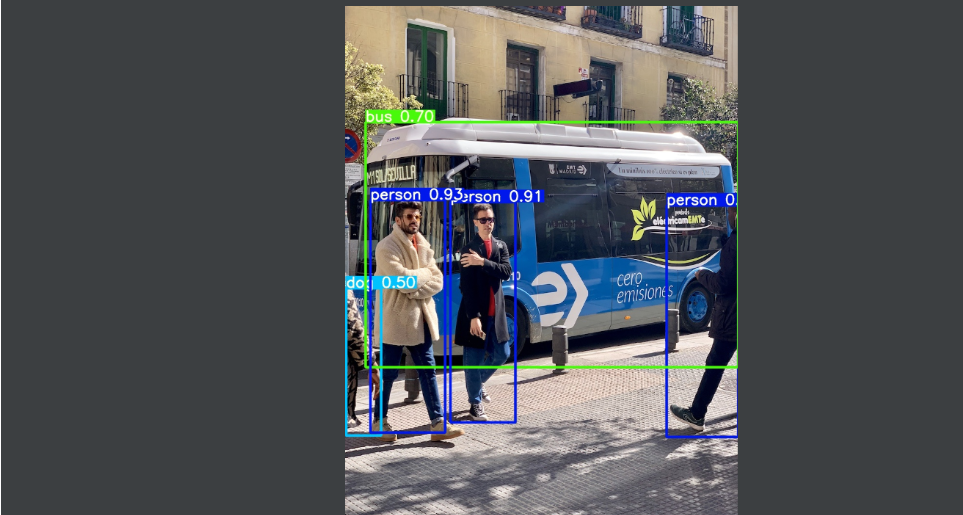
这个函数一般会用在detect.py中在nms之后变量每一个预测框,再将每个预测框画在原图上如:
                for *xyxy, conf, cls in reversed(det):
                    if save_txt:  # Write to file
                        xywh = (xyxy2xywh(torch.tensor(xyxy).view(1, 4)) / gn).view(-1).tolist()  # normalized xywh
                        line = (cls, *xywh, conf) if opt.save_conf else (cls, *xywh)  # label format
                        with open(txt_path + '.txt', 'a') as f:
                            f.write(('%g ' * len(line)).rstrip() % line + '\n')
效果如下所示:
2.2、plot_one_box_PIL(没用到)
这个函数是用PIL在原图中画一个框,作用和plot_one_box一样,而且我们一般都是用plot_one_box而不用这个函数,所以了解下即可。
plot_one_box_PIL函数代码:
def plot_one_box_PIL(box, im, color=(128, 128, 128), label=None, line_thickness=None):
    """
    使用PIL在原图im上画一个bounding box
    :params box: 预测得到的bounding box  [x1 y1 x2 y2]
    :params im: 原图 要将bounding box画在这个图上  array
    :params color: bounding box线的颜色
    :params label: 标签上的bounding box框框信息  类别 + score
    :params line_thickness: bounding box的线宽
    """
    # 将原图array格式->Image格式
    im = Image.fromarray(im)
    # (初始化)创建一个可以在给定图像(im)上绘图的对象, 在之后调用draw.函数的时候不需要传入im参数,它是直接针对im上进行绘画的
    draw = ImageDraw.Draw(im)
    # 设置绘制bounding box的线宽
    line_thickness = line_thickness or max(int(min(im.size) / 200), 2)
    # 在im图像上绘制bounding box
    # xy: box [x1 y1 x2 y2] 左上角 + 右下角  width: 线宽  outline: 矩形外框颜色color  fill: 将整个矩形填充颜色color
    # outline和fill一般根据需求二选一
    draw.rectangle(box, width=line_thickness, outline=color)  # plot
    # 如果label不为空还要在框框上面显示标签label + score
    if label:
        # 加载一个TrueType或者OpenType字体文件("Arial.ttf"), 并且创建一个字体对象font, font写出的字体大小size=12
        font = ImageFont.truetype("Arial.ttf", size=max(round(max(im.size) / 40), 12))
        # 返回给定文本label的宽度txt_width和高度txt_height
        txt_width, txt_height = font.getsize(label)
        # 在im图像上绘制矩形框 整个框框填充颜色color(用来存放label信息)  [x1 y1 x2 y2]  左上角 + 右下角
        draw.rectangle([box[0], box[1] - txt_height + 4, box[0] + txt_width, box[1]], fill=color)
        # 在上面这个矩形中写入text信息(label)  x1y1 左上角
        draw.text((box[0], box[1] - txt_height + 1), label, fill=(255, 255, 255), font=font)

    # 再返回array类型的im(绘好bounding box和label的)
    return np.asarray(im)
3、plot_wh_methods(没用到)
yolo.py:
 y = x[i].sigmoid()
 y[..., 0:2] = (y[..., 0:2] * 2. - 0.5 + self.grid[i]) * self.stride[i]  # xy
 y[..., 2:4] = (y[..., 2:4] * 2) ** 2 * self.anchor_grid[i]  # wh
 z.append(y.view(bs, -1, self.no))
loss.py:
# Regression
pxy = ps[:, :2].sigmoid() * 2. - 0.5
pwh = (ps[:, 2:4].sigmoid() * 2) ** 2 * anchors[i]
pbox = torch.cat((pxy, pwh), 1)  # predicted box
iou = bbox_iou(pbox.T, tbox[i], x1y1x2y2=False, CIoU=True)  # iou(prediction, target)
lbox += (1.0 - iou).mean()  # iou loss
plot_wh_methods函数代码:
def plot_wh_methods():
"""没用到
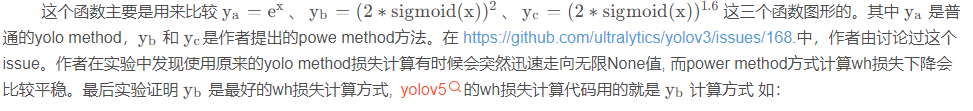
比较ya=e^x、yb=(2 * sigmoid(x))^2 以及 yc=(2 * sigmoid(x))^1.6 三个图形
wh损失计算的方式ya、yb、yc三种 ya: yolo method yb/yc: power method
实验发现使用原来的yolo method损失计算有时候会突然迅速走向无限None值, 而power method方式计算wh损失下降会比较平稳
最后实验证明yb是最好的wh损失计算方式, yolov5的wh损失计算代码用的就是yb计算方式
Compares the two methods for width-height anchor multiplication
https://github.com/ultralytics/yolov3/issues/168
"""
x = np.arange(-4.0, 4.0, .1) # (-4.0, 4.0) 每隔0.1取一个值
ya = np.exp(x) # ya = e^x yolo method
yb = torch.sigmoid(torch.from_numpy(x)).numpy() * 2 # yb = 2 * sigmoid(x)
fig = plt.figure(figsize=(6, 3), tight_layout=True) # 创建自定义图像 初始化画布
plt.plot(x, ya, '.-', label='YOLOv3') # 绘制折线图 可以任意加几条线
plt.plot(x, yb ** 2, '.-', label='YOLOv5 ^2')
plt.plot(x, yb ** 1.6, '.-', label='YOLOv5 ^1.6')
plt.xlim(left=-4, right=4) # 设置x轴、y轴范围
plt.ylim(bottom=0, top=6)
plt.xlabel('input') # 设置x轴、y轴标签
plt.ylabel('output')
plt.grid() # 生成网格
plt.legend() # 加上图例 如果是折线图,需要在plt.plot中加入label参数(图例名)
fig.savefig('comparison.png', dpi=200) # plt绘完图, fig.savefig()保存图片
其实这个函数倒不是特别重要,只是可视化一下这三个函数,看看他们的区别,在代码中也没调用过这个函数。但是了解这种新型 wh 损失计算的方式(Power Method)还是很有必要的。
4、output_to_target、plot_images
这两个函数其实也是对检测到的目标格式进行处理(output_to_target)然后再将其画框显示在原图上(plot_images)。不过这两个函数是用在test.py中的,针对的也不再是一张图片一个框,而是整个batch中的所有框。而且plot_images会将整个batch的图片都画在一张大图mosaic中,画不下的就删除。这些都是plot_images函数和plot_one_box的区别。
4.1、output_to_target
这个函数是用于将经过nms后的output [num_obj,x1y1x2y2+conf+cls] -> [num_obj,batch_id+class+xywh+conf]。并不涉及画图操作,而是转化predict的格式,通常放在画图操作plot_images之前。
output_to_target函数代码:
def output_to_target(output):
    """用在test.py中进行绘制前3个batch的预测框predictions 因为只有predictions需要修改格式 target是不需要修改格式的
    将经过nms后的output [num_obj,x1y1x2y2+conf+cls] -> [num_obj, batch_id+class+x+y+w+h+conf] 转变格式
    以便在plot_images中进行绘图 + 显示label
    Convert model output to target format [batch_id, class_id, x, y, w, h, conf]
    :params output: list{tensor(8)}分别对应着当前batch的8(batch_size)张图片做完nms后的结果
                    list中每个tensor[n, 6]  n表示当前图片检测到的目标个数  6=x1y1x2y2+conf+cls
    :return np.array(targets): [num_targets, batch_id+class+xywh+conf]  其中num_targets为当前batch中所有检测到目标框的个数
    """
    targets = []
    for i, o in enumerate(output):   # 对每张图片分别做处理
        for *box, conf, cls in o.cpu().numpy():  # 对每张图片的每个检测到的目标框进行convert格式
            targets.append([i, cls, *list(*xyxy2xywh(np.array(box)[None])), conf])
    return np.array(targets)
4.1、plot_images
这个函数是用来绘制一个batch的所有图片的框框(真实框或预测框)。使用在test.py中,且在output_to_target函数之后。而且这个函数是将一个batch的图片都放在一个大图mosaic上面,放不下删除。
plot_images函数代码:
def plot_images(images, targets, paths=None, fname='images.jpg', names=None, max_size=640, max_subplots=16):
"""用在test.py中进行绘制前3个batch的ground truth和预测框predictions(两个图) 一起保存 或者train.py中
将整个batch的labels都画在这个batch的images上
Plot image grid with labels
:params images: 当前batch的所有图片 Tensor [batch_size, 3, h, w] 且图片都是归一化后的
:params targets: 直接来自target: Tensor[num_target, img_index+class+xywh] [num_target, 6]
来自output_to_target: Tensor[num_pred, batch_id+class+xywh+conf] [num_pred, 7]
:params paths: tuple 当前batch中所有图片的地址
如: '..\\datasets\\coco128\\images\\train2017\\000000000315.jpg'
:params fname: 最终保存的文件路径 + 名字 runs\train\exp8\train_batch2.jpg
:params names: 传入的类名 从class index可以相应的key值 但是默认是None 只显示class index不显示类名
:params max_size: 图片的最大尺寸640 如果images有图片的大小(w/h)大于640则需要resize 如果都是小于640则不需要resize
:params max_subplots: 最大子图个数 16
:params mosaic: 一张大图 最多可以显示max_subplots张图片 将总多的图片(包括各自的label框框)一起贴在一起显示
mosaic每张图片的左上方还会显示当前图片的名字 最好以fname为名保存起来
"""
if isinstance(images, torch.Tensor):
images = images.cpu().float().numpy() # tensor -> numpy array
if isinstance(targets, torch.Tensor):
targets = targets.cpu().numpy()
# 反归一化 将归一化后的图片还原 un-normalise
if np.max(images[0]) <= 1:
images *= 255
# 设置一些基础变量
tl = 3 # 设置线宽 line thickness 3
tf = max(tl - 1, 1) # 设置字体笔画线宽 font thickness 2
bs, _, h, w = images.shape # batch size 4, channel 3, height 512, width 512
bs = min(bs, max_subplots) # 子图总数 正方形 limit plot images 4
ns = np.ceil(bs ** 0.5) # ns=每行/每列最大子图个数 子图总数=ns*ns ceil向上取整 2
# Check if we should resize
# 如果images有图片的大小(w/h)大于640则需要resize 如果都是小于640则不需要resize
scale_factor = max_size / max(h, w) # 1.25
if scale_factor < 1:
# 如果w/h有任何一条边超过640, 就要将较长边缩放到640, 另外一条边相应也缩放
h = math.ceil(scale_factor * h) # 512
w = math.ceil(scale_factor * w) # 512
# np.full 返回一个指定形状、类型和数值的数组
# shape: (int(ns * h), int(ns * w), 3) (1024, 1024, 3) 填充的值: 255 dtype 填充类型: np.uint8
mosaic = np.full((int(ns * h), int(ns * w), 3), 255, dtype=np.uint8) # init
# 对batch内每张图片
for i, img in enumerate(images): # img (3, 512, 512)
# 如果图片要超过max_subplots我们就不管了
if i == max_subplots: # if last batch has fewer images than we expect
break
# (block_x, block_y) 相当于是左上角的左边
block_x = int(w * (i // ns)) # // 取整 0 0 512 512 ns=2
block_y = int(h * (i % ns)) # % 取余 0 512 0 512
img = img.transpose(1, 2, 0) # (512, 512, 3) h w c
if scale_factor < 1: # 如果scale_factor < 1说明h/w超过max_size 需要resize回来
img = cv2.resize(img, (w, h))
# 将这个batch的图片一张张的贴到mosaic相应的位置上 hwc 这里最好自己画个图理解下
# 第一张图mosaic[0:512, 0:512, :] 第二张图mosaic[512:1024, 0:512, :]
# 第三张图mosaic[0:512, 512:1024, :] 第四张图mosaic[512:1024, 512:1024, :]
mosaic[block_y:block_y + h, block_x:block_x + w, :] = img
if len(targets) > 0:
# 求出属于这张img的target
image_targets = targets[targets[:, 0] == i]
# 将这张图片的所有target的xywh -> xyxy
boxes = xywh2xyxy(image_targets[:, 2:6]).T
# 得到这张图片所有target的类别classes
classes = image_targets[:, 1].astype('int')
# 如果image_targets.shape[1] == 6则说明没有置信度信息(此时target实际上是真实框)
# 如果长度为7则第7个信息就是置信度信息(此时target为预测框信息)
labels = image_targets.shape[1] == 6 # labels if no conf column
# 得到当前这张图的所有target的置信度信息(pred) 如果没有就为空(真实label)
# check for confidence presence (label vs pred)
conf = None if labels else image_targets[:, 6]
if boxes.shape[1]: # boxes.shape[1]不为空说明这张图有target目标
if boxes.max() <= 1.01: # if normalized with tolerance 0.01
# 因为图片是反归一化的 所以这里boxes也反归一化
boxes[[0, 2]] *= w # scale to pixels
boxes[[1, 3]] *= h
elif scale_factor < 1:
# 如果scale_factor < 1 说明resize过, 那么boxes也要相应变化
# absolute coords need scale if image scales
boxes *= scale_factor
# 上面得到的boxes信息是相对img这张图片的标签信息 因为我们最终是要将img贴到mosaic上 所以还要变换label->mosaic
boxes[[0, 2]] += block_x
boxes[[1, 3]] += block_y
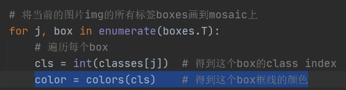
# 将当前的图片img的所有标签boxes画到mosaic上
for j, box in enumerate(boxes.T):
# 遍历每个box
cls = int(classes[j]) # 得到这个box的class index
color = colors(cls) # 得到这个box框线的颜色
cls = names[cls] if names else cls # 如果传入类名就显示类名 如果没传入类名就显示class index
# 如果labels不为空说明是在显示真实target 不需要conf置信度 直接显示label即可
# 如果conf[j] > 0.25 首先说明是在显示pred 且这个box的conf必须大于0.25 相当于又是一轮nms筛选 显示label + conf
if labels or conf[j] > 0.25: # 0.25 conf thresh
label = '%s' % cls if labels else '%s %.1f' % (cls, conf[j]) # 框框上面的显示信息
plot_one_box(box, mosaic, label=label, color=color, line_thickness=tl) # 一个个的画框
# 在mosaic每张图片相对位置的左上角写上每张图片的文件名 如000000000315.jpg
if paths:
# paths[i]: '..\\datasets\\coco128\\images\\train2017\\000000000315.jpg' Path: str -> Wins地址
# .name: str'000000000315.jpg' [:40]取前40个字符 最终还是等于str'000000000315.jpg'
label = Path(paths[i]).name[:40] # trim to 40 char
# 返回文本 label 的宽高 (width, height)
t_size = cv2.getTextSize(label, 0, fontScale=tl / 3, thickness=tf)[0]
# 在mosaic上写文本信息
# 要绘制的图像 + 要写上前的文本信息 + 文本左下角坐标 + 要使用的字体 + 字体缩放系数 + 字体的颜色 + 字体的线宽 + 矩形边框的线型
cv2.putText(mosaic, label, (block_x + 5, block_y + t_size[1] + 5), 0,
tl / 3, [220, 220, 220], thickness=tf, lineType=cv2.LINE_AA)
# mosaic内每张图片与图片之间弄一个边界框隔开 好看点 其实做法特简单 就是将每个img在mosaic中画个框即可
cv2.rectangle(mosaic, (block_x, block_y), (block_x + w, block_y + h), (255, 255, 255), thickness=3)
# 最后一步 check是否需要将mosaic图片保存起来
if fname: # 文件名不为空的话 fname = runs\train\exp8\train_batch2.jpg
# 限制mosaic图片尺寸
r = min(1280. / max(h, w) / ns, 1.0) # ratio to limit image size
mosaic = cv2.resize(mosaic, (int(ns * w * r), int(ns * h * r)), interpolation=cv2.INTER_AREA)
# cv2.imwrite(fname, cv2.cvtColor(mosaic, cv2.COLOR_BGR2RGB)) # cv2 save 最好BGR -> RGB再保存
Image.fromarray(mosaic).save(fname) # PIL save 必须要numpy array -> tensor格式 才能保存
return mosaic
这两个函数都是用在test.py函数中的:
用在train.py: